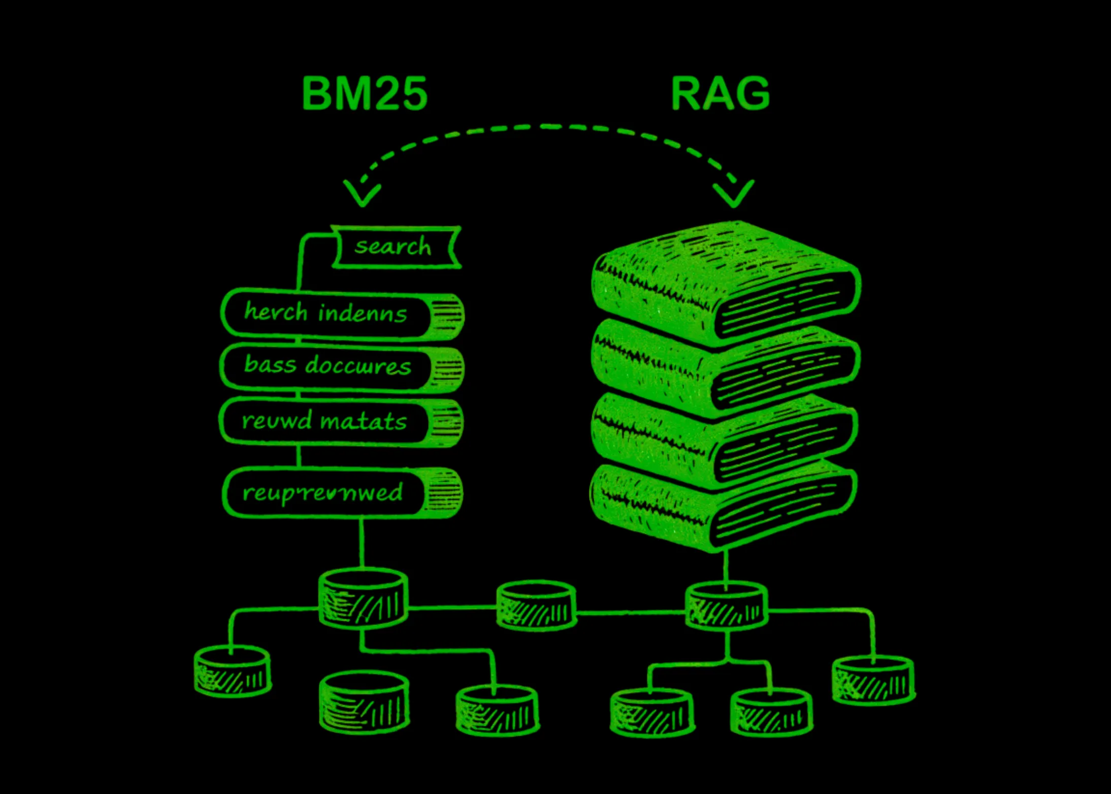
When you type a query into a search engine, something has to decide which documents are actually relevant — and how to rank them. BM25 (Best Matching 25), the algorithm powering search engines like Elasticsearch and Lucene, has been the dominant answer to that question for decades.
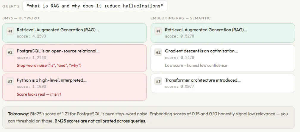
It scores documents by looking at three things: how often your query terms appear in a document, how rare those terms are across the entire collection, and whether a document is unusually long. The clever part is that BM25 doesn’t reward keyword stuffing — a word appearing 20 times doesn’t make a document 20 times more relevant, thanks to term frequency saturation. But BM25 has a fundamental blind spot: it only matches the words you typed, not what you meant. Search for “finding similar content without exact word overlap” and BM25 returns a blank stare.
This is exactly the gap that Retrieval-Augmented Generation (RAG) with vector embeddings was built to fill — by matching meaning, not just keywords. In this article, we’ll break down how each approach works, where each one wins, and why production systems increasingly use both together.
How BM25 Works
At its core, BM25 assigns a relevance score to every document in the collection for a given query, then ranks documents by that score. For each term in your query, BM25 asks three questions: How often does this term appear in the document? How rare is this term across all documents? And is this document unusually long? The final score is the sum of weighted answers to these questions across all query terms.
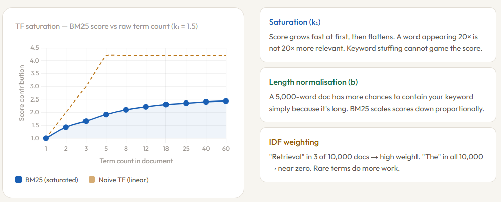
The term frequency component is where BM25 gets clever. Rather than counting raw occurrences, it applies saturation — the score grows quickly at first but flattens out as frequency increases. A term appearing 5 times contributes much more than a term appearing once, but a term appearing 50 times contributes barely more than one appearing 20 times. This is controlled by the parameter k₁ (typically set between 1.2 and 2.0). Set it low and the saturation kicks in fast; set it high and raw frequency matters more. This single design choice is what makes BM25 resistant to keyword stuffing — repeating a word a hundred times in a document won’t game the score.
Length Normalization and IDF
The second tuning parameter, b (typically 0.75), controls how much a document’s length is penalized. A long document naturally contains more words, so it has more chances to include your query term — not because it’s more relevant, but simply because it’s longer. BM25 compares each document’s length to the average document length in the collection and scales the term frequency score down accordingly. Setting b = 0 disables this penalty entirely; b = 1 applies full normalization.
Finally, IDF (Inverse Document Frequency) ensures that rare terms carry more weight than common ones. If the word “retrieval” appears in only 3 out of 10,000 documents, it’s a strong signal of relevance when matched. If the word “the” appears in all 10,000, matching it tells you almost nothing. IDF is what makes BM25 pay attention to the words that actually discriminate between documents. One important caveat: because BM25 operates purely on term frequency, it has no awareness of word order, context, or meaning — matching “bank” in a query about finance and “bank” in a document about rivers looks identical to BM25. That bag-of-words limitation is fundamental, not a tuning problem.
How is BM25 different from Vector Search
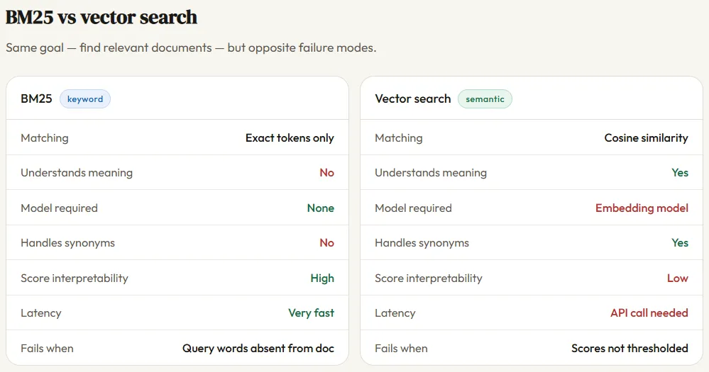
BM25 and vector search answer the same question — which documents are relevant to this query? — but through fundamentally different lenses. BM25 is a keyword-matching algorithm: it looks for the exact words from your query inside each document, scores them based on frequency and rarity, and ranks accordingly. It has no understanding of language — it sees text as a bag of tokens, not meaning.
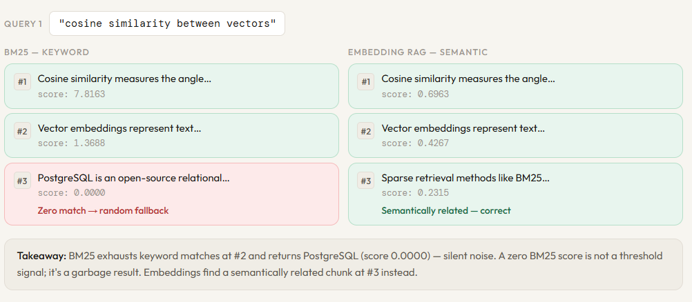
Vector search, by contrast, converts both the query and every document into dense numerical vectors using an embedding model, then finds documents whose vectors point in the same direction as the query vector — measured by cosine similarity. This means vector search can match “cardiac arrest” to a document about “heart failure” even though none of the words overlap, because the embedding model has learned that these concepts live close together in semantic space.
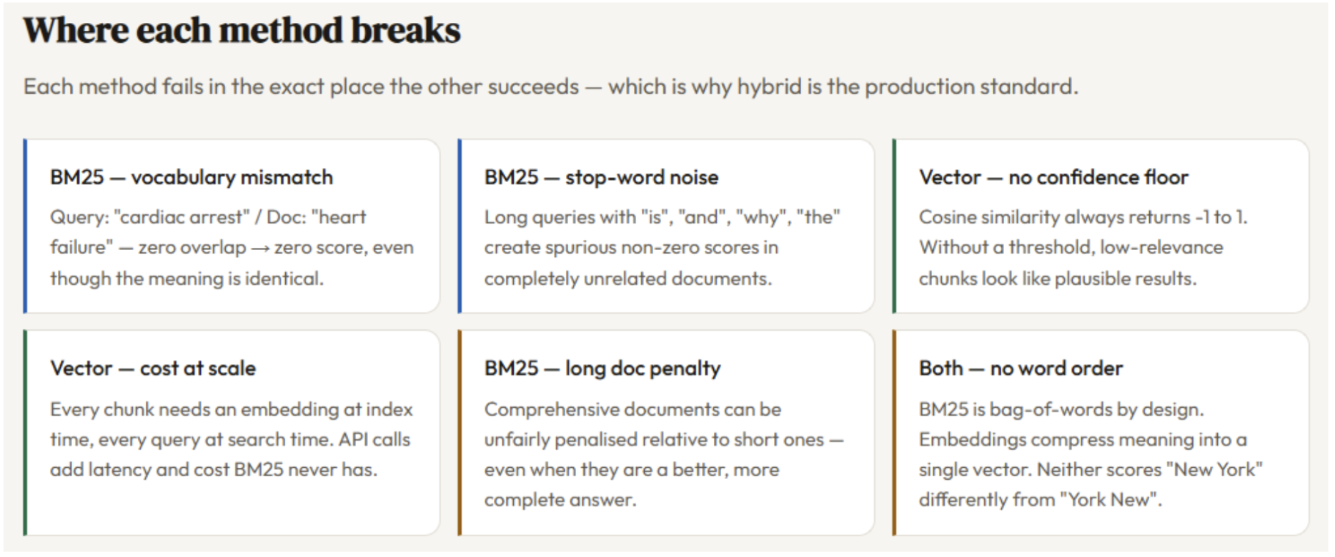
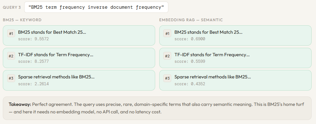
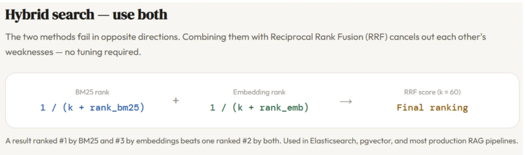
The tradeoff is practical: BM25 requires no model, no GPU, and no API call — it’s fast, lightweight, and fully explainable. Vector search requires an embedding model at index time and query time, adds latency and cost, and produces scores that are harder to interpret. Neither is strictly better; they fail in opposite directions, which is exactly why hybrid search — combining both — has become the production standard.
Comparing BM25 and Vector Search in Python
Installing the dependencies
import re
import numpy as np
from collections import Counter
from rank_bm25 import BM25Okapi
from openai import OpenAI
from getpass import getpass
os.environ[‘OPENAI_API_KEY’] = getpass(‘Enter OpenAI API Key: ‘)
Defining the Corpus
Before comparing BM25 and vector search, we need a shared knowledge base to search over. We define 12 short text chunks covering a range of topics — Python, machine learning, BM25, transformers, embeddings, RAG, databases, and more. The topics are deliberately varied: some chunks are closely related (BM25 and TF-IDF, embeddings and cosine similarity), while others are completely unrelated (PostgreSQL, Django). This variety is what makes the comparison meaningful — a retrieval method that works well should surface the relevant chunks and ignore the noise.
This corpus acts as our stand-in for a real document store. In a production RAG pipeline, these chunks would come from splitting and cleaning actual documents — PDFs, wikis, knowledge bases. Here, we keep them short and hand-crafted so the retrieval behaviour is easy to trace and reason about.
# 0
“Python is a high-level, interpreted programming language known for its simple and readable syntax. ”
“It supports multiple programming paradigms including procedural, object-oriented, and functional programming.”,
# 1
“Machine learning is a subset of artificial intelligence that enables systems to learn from data ”
“without being explicitly programmed. Common algorithms include linear regression, decision trees, and neural networks.”,
# 2
“BM25 stands for Best Match 25. It is a bag-of-words retrieval function used by search engines ”
“to rank documents based on the query terms appearing in each document. ”
“BM25 uses term frequency and inverse document frequency with length normalization.”,
# 3
“Transformer architecture introduced the self-attention mechanism, which allows the model to weigh ”
“the importance of different words in a sentence regardless of their position. ”
“BERT and GPT are both based on the Transformer architecture.”,
# 4
“Vector embeddings represent text as dense numerical vectors in a high-dimensional space. ”
“Similar texts are placed closer together. This allows semantic search — finding documents ”
“that mean the same thing even if they use different words.”,
# 5
“TF-IDF stands for Term Frequency-Inverse Document Frequency. It reflects how important a word is ”
“to a document relative to the entire corpus. Rare words get higher scores than common ones like ‘the’.”,
# 6
“Retrieval-Augmented Generation (RAG) combines a retrieval system with a language model. ”
“The retriever finds relevant documents; the generator uses them as context to produce an answer. ”
“This reduces hallucinations and allows the model to cite sources.”,
# 7
“Django is a high-level Python web framework that encourages rapid development and clean, pragmatic design. ”
“It includes an ORM, authentication system, and admin panel out of the box.”,
# 8
“Cosine similarity measures the angle between two vectors. A score of 1 means identical direction, ”
“0 means orthogonal, and -1 means opposite. It is commonly used to compare text embeddings.”,
# 9
“Gradient descent is an optimization algorithm used to minimize a loss function by iteratively ”
“moving in the direction of the steepest descent. It is the backbone of training neural networks.”,
# 10
“PostgreSQL is an open-source relational database known for its robustness and support for advanced ”
“SQL features like window functions, CTEs, and JSON storage.”,
# 11
“Sparse retrieval methods like BM25 rely on exact keyword matches and fail when the query uses ”
“synonyms or paraphrases not present in the document. Dense retrieval using embeddings handles ”
“this by matching semantic meaning rather than surface form.”,
]
print(f”Corpus loaded: {len(CHUNKS)} chunks”)
for i, c in enumerate(CHUNKS):
print(f” [{i:02d}] {c[:75]}…”)
Building the BM25 Retriever
With the corpus defined, we can build the BM25 index. The process has two steps: tokenization and indexing. The tokenize function lowercases the text and splits on any non-alphanumeric character — so “TF-IDF” becomes [“tf”, “idf”] and “bag-of-words” becomes [“bag”, “of”, “words”]. This is intentionally simple: BM25 is a bag-of-words model, so there is no stemming, no stopword removal, and no linguistic preprocessing. Every word is treated as an independent token.
Once every chunk is tokenized, BM25Okapi builds the index — computing document lengths, average document length, and IDF scores for every unique term in the corpus. This happens once at startup. At query time, bm25_search tokenizes the incoming query the same way, calls get_scores to compute a BM25 relevance score for every chunk in parallel, then sorts and returns the top-k results. The sanity check at the bottom runs a test query to confirm the index is working before we move on to the embedding retriever.
“””Lowercase and split on non-alphanumeric characters.”””
return re.findall(r’\w+’, text.lower())
# Build BM25 index over the corpus
tokenized_corpus = [tokenize(chunk) for chunk in CHUNKS]
bm25 = BM25Okapi(tokenized_corpus)
def bm25_search(query: str, top_k: int = 3) -> list[dict]:
“””Return top-k chunks ranked by BM25 score.”””
tokens = tokenize(query)
scores = bm25.get_scores(tokens)
ranked = np.argsort(scores)[::-1][:top_k]
return [
{“chunk_id”: int(i), “score”: round(float(scores[i]), 4), “text”: CHUNKS[i]}
for i in ranked
]
# Quick sanity check
results = bm25_search(“how does BM25 rank documents”, top_k=3)
print(“BM25 test — query: ‘how does BM25 rank documents'”)
for r in results:
print(f” [{r[‘chunk_id’]}] score={r[‘score’]} {r[‘text’][:70]}…”)
Building the Embedding Retriever
The embedding retriever works differently from BM25 at every step. Instead of counting tokens, it converts each chunk into a dense numerical vector — a list of 1,536 numbers — using OpenAI’s text-embedding-3-small model. Each number represents a dimension in semantic space, and chunks that mean similar things end up with vectors that point in similar directions, regardless of the words they use.
The index build step calls the embedding API once per chunk and stores the resulting vectors in memory. This is the key cost difference from BM25: building the BM25 index is pure arithmetic on your own machine, while building the embedding index requires one API call per chunk and produces vectors you need to store. For 12 chunks this is trivial; at a million chunks, this becomes a real infrastructure decision.
At query time, embedding_search embeds the incoming query using the same model — this is important, the query and the chunks must live in the same vector space — then computes cosine similarity between the query vector and every stored chunk vector. Cosine similarity measures the angle between two vectors: a score of 1 means identical direction, 0 means completely unrelated, and negative values mean opposite meaning. The chunks are then ranked by this score and the top-k are returned. The same sanity check query from the BM25 section runs here too, so you can see the first direct comparison between the two approaches on identical input.
def get_embedding(text: str) -> np.ndarray:
response = client.embeddings.create(model=EMBED_MODEL, input=text)
return np.array(response.data[0].embedding)
def cosine_similarity(a: np.ndarray, b: np.ndarray) -> float:
return float(np.dot(a, b) / (np.linalg.norm(a) * np.linalg.norm(b)))
# Embed all chunks once (this is the “index build” step in RAG)
print(“Building embedding index… (one API call per chunk)”)
chunk_embeddings = [get_embedding(chunk) for chunk in CHUNKS]
print(f”Done. Each embedding has {len(chunk_embeddings[0])} dimensions.”)
def embedding_search(query: str, top_k: int = 3) -> list[dict]:
“””Return top-k chunks ranked by cosine similarity to the query embedding.”””
query_emb = get_embedding(query)
scores = [cosine_similarity(query_emb, emb) for emb in chunk_embeddings]
ranked = np.argsort(scores)[::-1][:top_k]
return [
{“chunk_id”: int(i), “score”: round(float(scores[i]), 4), “text”: CHUNKS[i]}
for i in ranked
]
# Quick sanity check
results = embedding_search(“how does BM25 rank documents”, top_k=3)
print(“\nEmbedding test — query: ‘how does BM25 rank documents'”)
for r in results:
print(f” [{r[‘chunk_id’]}] score={r[‘score’]} {r[‘text’][:70]}…”)
Side-by-Side Comparison Function
This is the core of the experiment. The compare function runs the same query through both retrievers simultaneously and prints the results in a two-column layout — BM25 on the left, embeddings on the right — so the differences are immediately visible at the same rank position.
bm25_results = bm25_search(query, top_k)
embed_results = embedding_search(query, top_k)
print(f”\n{‘═’*70}”)
print(f” QUERY: \”{query}\””)
print(f”{‘═’*70}”)
print(f”\n {‘BM25 (keyword)’:<35} {‘Embedding RAG (semantic)’}”)
print(f” {‘─’*33} {‘─’*33}”)
for rank, (b, e) in enumerate(zip(bm25_results, embed_results), 1):
b_preview = b[‘text’][:55].replace(‘\n’, ‘ ‘)
e_preview = e[‘text’][:55].replace(‘\n’, ‘ ‘)
same = “⬅ same” if b[‘chunk_id’] == e[‘chunk_id’] else “”
print(f” #{rank} [{b[‘chunk_id’]:02d}] {b[‘score’]:.4f} {b_preview}…”)
print(f” [{e[‘chunk_id’]:02d}] {e[‘score’]:.4f} {e_preview}… {same}”)
print()
compare(“what is RAG and why does it reduce hallucinations”)
compare(“cosine similarity between vectors”)
Check out the Full Notebook here. Also, feel free to follow us on Twitter and don’t forget to join our 120k+ ML SubReddit and Subscribe to our Newsletter. Wait! are you on telegram? now you can join us on telegram as well.

I am a Civil Engineering Graduate (2022) from Jamia Millia Islamia, New Delhi, and I have a keen interest in Data Science, especially Neural Networks and their application in various areas.